5. Running a full analysis

Written by Jin Hyun Cheong and Eshin Jolly

In this tutorial we’ll perform a real analysis on part of the open dataset from “A Data-Driven Characterisation Of Natural Facial Expressions When Giving Good And Bad News” by Watson & Johnston 2020. You can try it out interactively in Google Collab:

In the original paper the authors had 3 speakers deliver good or bad news while filming their facial expressions. They found that could accurately “decode” each condition based on participants’ facial expressions extracted either using a custom multi-chanel-gradient model or action units (AUs) extracted using Open Face.

In this tutorial we’ll show how easiy it is to not only reproduce their decoding analysis with py-feat, but just as easily perform additional analyses. Specifically we’ll:

1. Download 20 of the first subject’s videos (the full dataset is available on OSF

2. Extract facial features using the Detector

3. Aggregate and summarize detections per video using Fex

4. Train and test a decoder to classify good vs bad news using extracted emotions, AUs, and poses

5. Run a fMRI style “mass-univariate” comparison across all AUs between conditions

6. Run a time-series analysis comparing videos based on the time-courses of extracted facial fatures

# Uncomment the line below and run this only if you're using Google Collab
# !pip install -q py-feat

5.1 Download the data

Here’s we’ll download and save the first 20 video files and their corresponding attributes from OSF. The next cell should run quickly on Google Collab, but will depend on your own internet conection if you’re executing this notebook locally. You can rerun this cell in case the download fails for any reason, as it should skip downloading existing files:

import os
import subprocess
import numpy as np
import pandas as pd
import matplotlib.pyplot as plt
from glob import glob
import seaborn as sns
from tqdm import tqdm
sns.set_context("talk")

files_to_download = {
    "4c5mb": 'clip_attrs.csv',
    "n6rt3": '001.mp4',
    "3gh8v": '002.mp4',
    "twqxs": '003.mp4',
    "nc7d9": '004.mp4',
    "nrwcm": '005.mp4',
    "2rk9c": '006.mp4',
    "mxkzq": '007.mp4',
    "c2na7": '008.mp4',
    "wj7zy": '009.mp4',
    "mxywn": '010.mp4',
    "6bn3g": '011.mp4',
    "jkwsp": '012.mp4',
    "54gtv": '013.mp4',
    "c3hpm": '014.mp4',
    "utdqj": '015.mp4',
    "hpw4a": '016.mp4',
    "94swe": '017.mp4',
    "qte5y": '018.mp4',
    "aykvu": '019.mp4',
    "3d5ry": '020.mp4',
}

for fid, fname in files_to_download.items():
    if not os.path.exists(fname):
        print(f"Downloading: {fname}")
        subprocess.run(f"wget -O {fname} --content-disposition https://osf.io/{fid}/download".split())

videos = np.sort(glob("*.mp4"))

# Load in attributes
clip_attrs = pd.read_csv("clip_attrs.csv")

# Add in file names and rename conditions
clip_attrs = clip_attrs.assign(
    input=clip_attrs.clipN.apply(lambda x: str(x).zfill(3) + ".mp4"),
    condition=clip_attrs["class"].replace({"gn": "goodNews", "ists": "badNews"}),
)

# We're only using a subset of videos for this tutorial so drop the rest
clip_attrs = clip_attrs.query("input in @videos")

print(f"Downloaded {len(videos)} videos")
print(f"Downloaded attributes files with {clip_attrs.shape[0]} rows")

Downloaded 20 videos
Downloaded attributes files with 20 rows

5.2 Extract facial features using Detector

Now we’ll initialize a new Detector, process each frame of each video using .detect_video(), and save the results to csv files named after the video.

from feat import Detector

# Initialize the default detector
detector = Detector()

# Loop over and process each video and save results to csv
for video in tqdm(videos):
    out_name = video.replace(".mp4", ".csv")
    if not os.path.exists(out_name):

        print(f"Processing: {video}")

        # This is the line that does detection!
        fex = detector.detect_video(video)

        fex.to_csv(out_name, index=False)

5.3. Aggregate detections using a Fex dataframe

Then we can use read_feat to load each CSV file and concatenate them together:

from feat.utils.io import read_feat

fex = pd.concat(map(lambda video: read_feat(video.replace(".mp4", ".csv")), videos))

print(f"Unique videos: {fex.inputs.nunique()}")
print(f"Total processed frames: {fex.shape[0]}")
print(f"Avg frames per video: {fex.groupby('input').size().mean()}")

Unique videos: 20
Total processed frames: 947
Avg frames per video: 47.35

Our Fex dataframe now contains all detections for all frames of each video

fex.shape
fex.head()

(947, 174)

	FaceRectX	FaceRectY	FaceRectWidth	FaceRectHeight	FaceScore	x_0	x_1	x_2	x_3	x_4	...	anger	disgust	fear	happiness	sadness	surprise	neutral	input	frame	approx_time
0	364.351590	281.705972	393.321784	538.626011	0.999326	355.590267	361.166635	370.024031	382.002333	405.379242	...	0.000438	0.000117	0.000483	0.981574	0.001495	0.013396	0.002497	001.mp4	0	00:00
1	364.420098	281.698321	393.282234	538.731126	0.999327	355.947047	361.429636	370.189673	382.098332	405.381871	...	0.000422	0.000110	0.000471	0.981490	0.001407	0.013663	0.002437	001.mp4	1	00:00
2	366.712348	280.100516	393.075675	538.872332	0.999371	357.488551	363.557662	372.905629	385.126006	408.333512	...	0.000379	0.000112	0.000329	0.988872	0.001477	0.006877	0.001954	001.mp4	2	00:00
3	369.679081	279.800566	392.800373	541.545800	0.999298	358.248297	364.062520	373.173968	385.128103	407.907217	...	0.000451	0.000122	0.000229	0.989229	0.001519	0.005104	0.003346	001.mp4	3	00:00
4	368.641343	273.729074	397.080568	550.337162	0.999240	353.728640	360.555682	370.127252	382.294048	405.861680	...	0.000388	0.000067	0.000447	0.976272	0.001275	0.016979	0.004573	001.mp4	4	00:00

5 rows × 174 columns

5.3.1 Summarize data with Fex.sessions

Fex dataframes have a special attribute called .sessions that act as a grouping factor to make it easier to compute summary statistics with any of the .extract_* methods. By default .sessions is None, but you can use the .update_sessions() to return a new Fex dataframe with .sessions set.

For example, if we update the sessions to be the name of each video, then .extract_mean() will group video-frames (rows) by video making it easy to compute a single summary statistic per file:

by_video = fex.update_sessions(fex["input"])

# Compute the mean per video
video_means = by_video.extract_mean()

video_means # 20 rows for 20 videos

	mean_FaceRectX	mean_FaceRectY	mean_FaceRectWidth	mean_FaceRectHeight	mean_FaceScore	mean_x_0	mean_x_1	mean_x_2	mean_x_3	mean_x_4	...	mean_AU28	mean_AU43	mean_anger	mean_disgust	mean_fear	mean_happiness	mean_sadness	mean_surprise	mean_neutral	mean_frame
001.mp4	361.693876	276.801922	390.643836	538.546526	0.999415	351.745947	358.669057	369.211596	382.289621	405.340749	...	0.400157	0.078763	0.000840	0.000170	0.002119	0.955028	0.011139	0.022887	0.007818	19.5
002.mp4	362.782907	273.463460	381.666967	534.798252	0.999420	351.152403	356.936973	366.408657	378.847147	401.092449	...	0.310074	0.123018	0.000609	0.000115	0.001898	0.879776	0.012571	0.094248	0.010782	13.5
003.mp4	356.546617	271.015871	388.101834	541.721541	0.999401	342.375212	346.903972	354.548829	365.250301	386.696666	...	0.263471	0.037146	0.000355	0.000061	0.001733	0.707242	0.001066	0.285287	0.004256	23.0
004.mp4	340.658119	271.997003	390.052859	545.905496	0.999425	328.644936	334.260224	342.829941	354.501717	376.853730	...	0.264972	0.099364	0.000721	0.000068	0.001341	0.847641	0.012390	0.132939	0.004900	22.0
005.mp4	322.252894	292.223503	393.885578	539.983786	0.999394	312.148711	317.922322	327.292733	339.933222	363.364786	...	0.366397	0.132650	0.000226	0.000043	0.000490	0.986752	0.001082	0.009684	0.001723	22.0
006.mp4	351.829324	263.138842	383.265317	541.386626	0.999457	339.691768	343.841731	351.142231	361.316873	382.081545	...	0.366849	0.059786	0.000246	0.000036	0.000628	0.941467	0.001282	0.054525	0.001816	23.5
007.mp4	358.451365	267.047528	385.200341	539.094825	0.999380	345.372773	348.641482	355.122228	364.639966	384.731837	...	0.326419	0.043416	0.000374	0.000058	0.002243	0.933058	0.003285	0.057281	0.003701	13.0
008.mp4	335.531841	269.932394	389.309414	543.007503	0.999335	322.590086	328.698168	337.769330	348.969558	369.878785	...	0.482863	0.037955	0.000327	0.000091	0.004953	0.592064	0.003459	0.393644	0.005462	17.5
009.mp4	341.377368	258.612550	384.471775	547.748099	0.999307	328.585905	334.560713	343.619836	355.424001	377.394425	...	0.428292	0.048874	0.000317	0.000195	0.014244	0.536781	0.003003	0.442032	0.003427	20.5
010.mp4	350.612259	285.415234	382.804314	537.392594	0.999450	336.439669	342.711365	352.625989	365.147914	388.132257	...	0.452048	0.068882	0.000243	0.000051	0.005075	0.691970	0.008150	0.290069	0.004443	26.5
011.mp4	342.846589	323.818531	380.793417	537.407032	0.999462	317.001702	329.615415	347.071755	367.541387	397.147639	...	0.382106	0.053013	0.130460	0.007293	0.067473	0.134826	0.119239	0.239828	0.300882	17.5
012.mp4	346.793633	345.102172	376.265186	526.341481	0.999400	321.367646	334.862112	352.977879	374.908646	405.053755	...	0.308746	0.191442	0.002793	0.001974	0.073120	0.066317	0.176804	0.657999	0.020993	23.5
013.mp4	353.966822	291.357734	381.017808	541.329173	0.999402	341.007234	351.553327	365.335356	382.232456	408.826613	...	0.471486	0.040775	0.001247	0.000341	0.027139	0.025583	0.140288	0.772149	0.033251	13.5
014.mp4	349.458311	277.770594	378.477618	543.834237	0.999373	326.507088	338.703004	355.255419	375.844798	405.824674	...	0.320477	0.036352	0.004123	0.002852	0.259469	0.000338	0.242996	0.452750	0.037473	22.0
015.mp4	341.266907	300.009642	376.853981	540.635116	0.999404	318.571982	329.832546	345.395775	364.710552	393.250724	...	0.245678	0.134054	0.001375	0.000311	0.195097	0.003530	0.434903	0.350142	0.014644	29.0
016.mp4	311.328833	290.488594	383.377662	533.601522	0.999459	297.753369	309.231162	324.626972	343.137091	370.771578	...	0.408074	0.042457	0.002659	0.001119	0.053669	0.005470	0.150112	0.737356	0.049615	38.5
017.mp4	332.626607	301.264397	381.029439	528.518111	0.999355	323.741976	329.358193	338.566349	351.548930	373.243177	...	0.271463	0.037381	0.000944	0.000358	0.061095	0.006041	0.050949	0.866098	0.014514	28.0
018.mp4	353.881611	288.094093	379.735909	543.683842	0.999429	328.829019	337.406731	350.572361	368.037250	395.964752	...	0.328093	0.033050	0.007092	0.002789	0.155484	0.012824	0.175173	0.519115	0.127522	26.5
019.mp4	313.341504	282.379830	391.049851	543.151199	0.999275	303.143011	310.439069	321.088562	334.650816	358.007455	...	0.364117	0.040580	0.000663	0.000140	0.116914	0.000767	0.374723	0.490313	0.016481	31.5
020.mp4	303.021553	287.952208	385.861488	524.438969	0.999489	293.626183	302.517683	314.678548	329.424593	353.108089	...	0.322978	0.040657	0.000776	0.000236	0.086137	0.014581	0.059977	0.822615	0.015677	32.5

20 rows × 172 columns

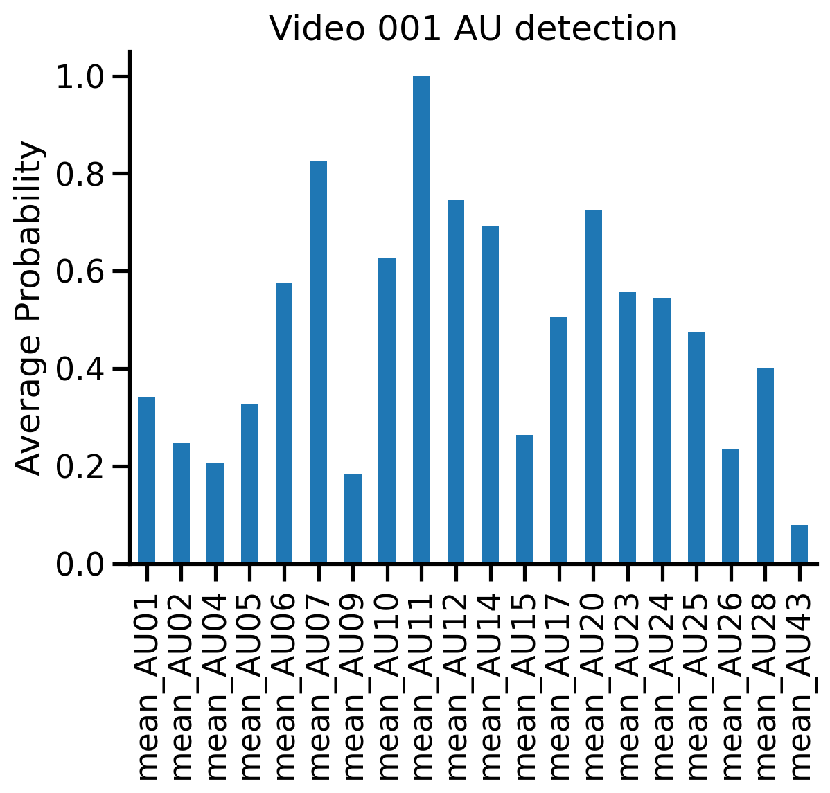
Then we can grab the AU detections and call standard pandas methods like .loc and .plot:

# Grab the aus just for video 1
video001_aus = video_means.aus.loc['001.mp4']
# video001_aus = video_means.aus.loc['001.csv'] # if loading pre-computed csv

# Plot them
ax = video001_aus.plot(kind='bar', title='Video 001 AU detection');
ax.set(ylabel='Average Probability');
sns.despine();

5.3.2 Chaining operations

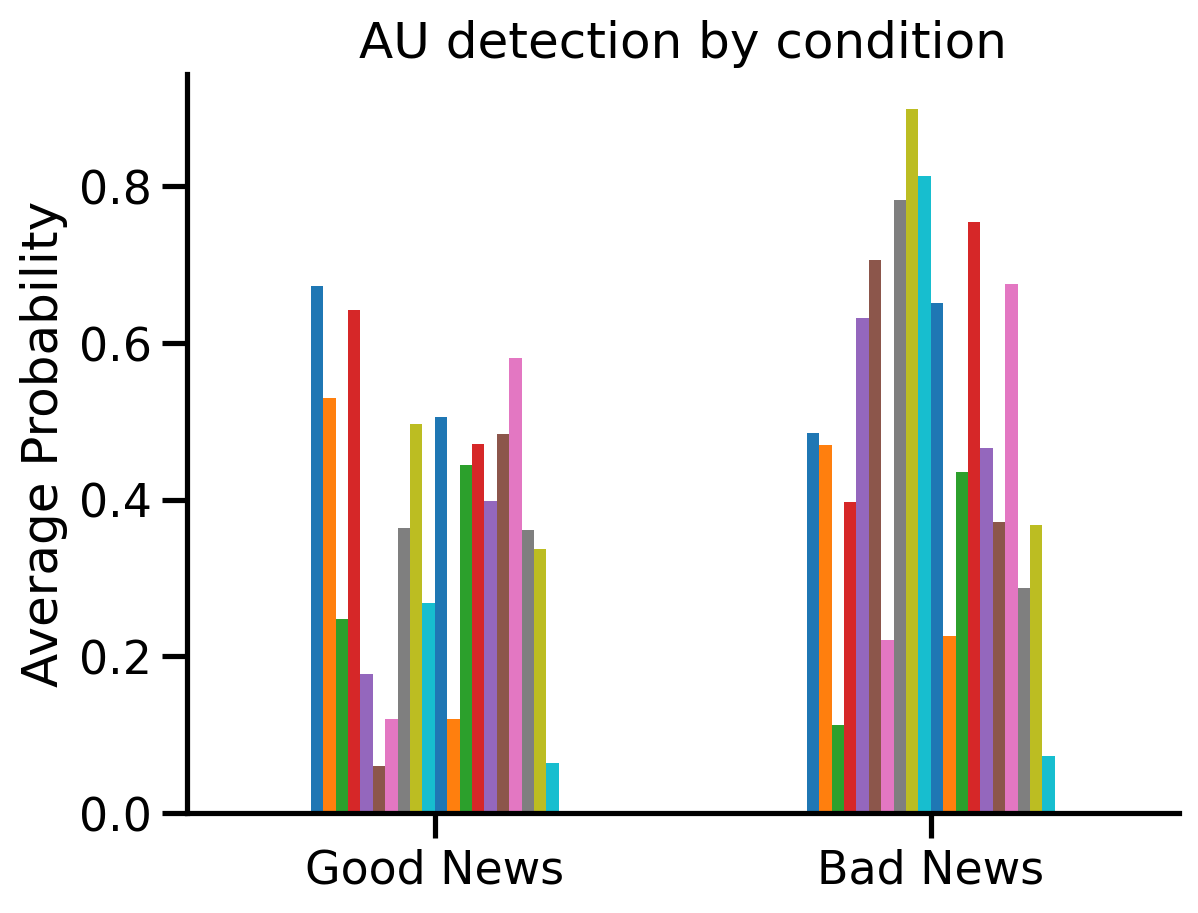
.update_sessions() always returns a copy of the Fex object, so that you can chain operations together including existing pandas methods like .plot(). Here’s an example passing a dictionary to .update_sessions(), which maps between old and new session names:

# Which condition each video belonged to
video2condition = dict(
    zip(
        # if loading pre-computed csv
        # clip_attrs["input"].str.replace(".mp4", ".csv", regex=False),
        clip_attrs["input"],
        clip_attrs["condition"],
    )
)

# Update sesssions to group by condition, compute means (per condition), and make a
# barplot of the mean AUs for each condition
ax = (
    by_video.update_sessions(video2condition)
    .extract_mean()
    .aus.plot(kind="bar", legend=False, title="Mean AU detection by condition")
)
ax.set(ylabel='Average Probability', title='AU detection by condition', xticklabels=['Good News', 'Bad News']);
plt.xticks(rotation=0);
sns.despine();

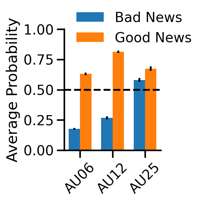
We can also focus in on the AUs associated with happiness:

aus = ["AU06", "AU12", "AU25"]  # from https://py-feat.org/pages/au_reference.html

# Update the sessions to condition compute summary stats
summary = by_video.update_sessions(video2condition).extract_summary(
    mean=True, sem=True, std=False, min=False, max=False
)

# Organize them for plotting
bad_means = summary.loc["badNews", [f"mean_{au}" for au in aus]]
bad_sems = summary.loc["badNews", [f"sem_{au}" for au in aus]]
good_means = summary.loc["goodNews", [f"mean_{au}" for au in aus]]
good_sems = summary.loc["goodNews", [f"sem_{au}" for au in aus]]

# Plot
fig, ax = plt.subplots(figsize=(3, 4))
ind = np.arange(len(bad_means))
width = 0.35
rects1 = ax.bar(ind - width / 2, bad_means, width, yerr=bad_sems, label="Bad News");
rects2 = ax.bar(ind + width / 2, good_means, width, yerr=good_sems, label="Good News");
ax.set(ylabel="Average Probability", title="", xticks=ind, xticklabels=aus, ylim=(0, 1));
ax.legend(loc="upper left", frameon=False, bbox_to_anchor=(0, 1.25));
plt.axhline(0.5, ls="--", color="k");
sns.despine();
plt.xticks(rotation=45);
plt.tight_layout();
plt.savefig('./fig_maker/au_diffs.pdf', bbox_inches='tight');

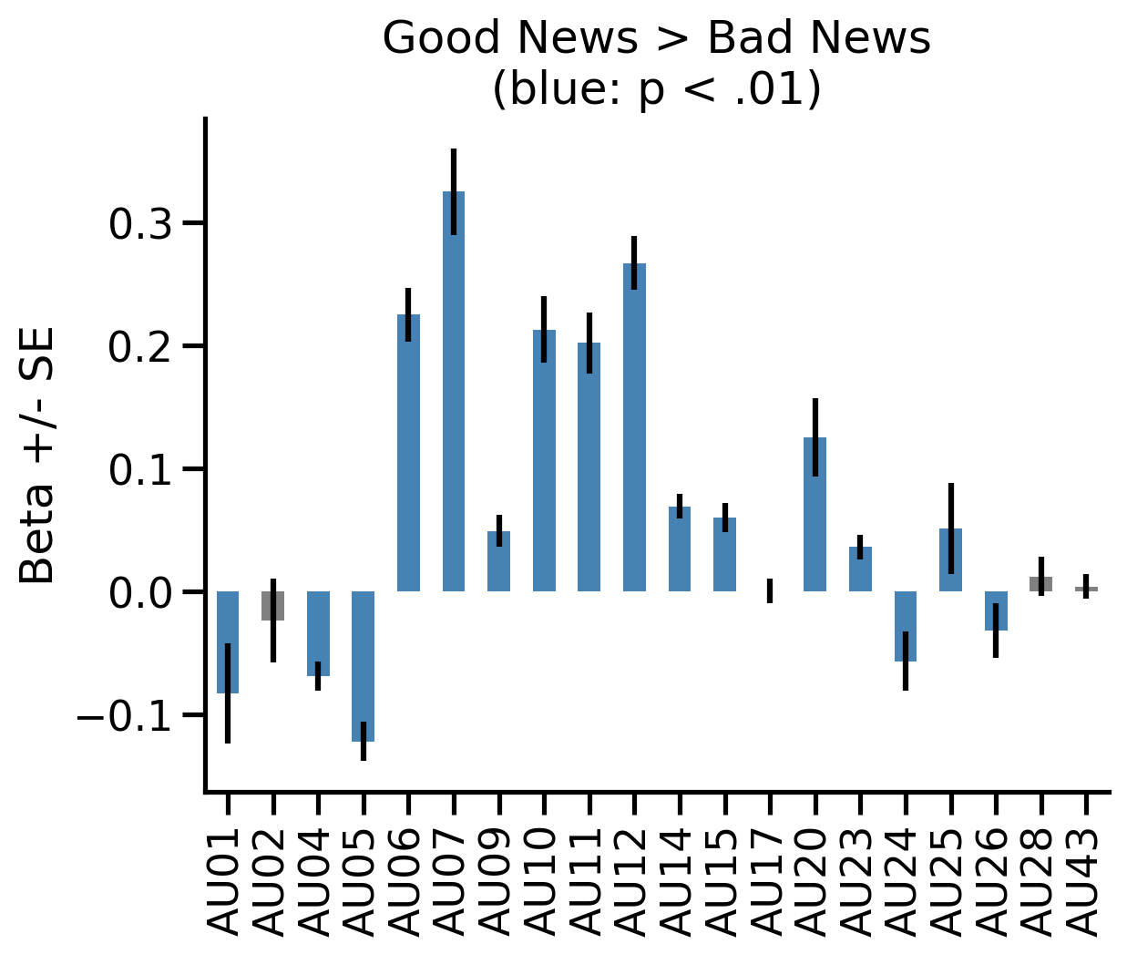
5.4 Comparing the condition difference across AUs using regression

One way we can compare what AUs in the plot show significant differences is by using the .regress() method along with numerical contrast codes. For example we can test the difference in activation of every AU when participants delivered good vs bad news.

This is analogous to the “mass-univariate” GLM approach in fMRI research, and allows us to identify what AUs are significantly more active in one condition vs another:

# Save the by_condition fex from above
by_condition = video_means.update_sessions(video2condition)

# We set numerical contrasts to compare mean good news > mean bad news
by_condition_codes = by_condition.update_sessions({"goodNews": 1., "badNews": -1})

# Now we perform a regression (t-test) at every AU
b, se, t, p, df, residuals = by_condition_codes.regress(
    X="sessions", y="aus", fit_intercept=True
)

# We can perform bonferroni correction for multiple comparisions:
p_bonf = p / p.shape[1]

results = pd.concat(
    [
        b.round(3).loc[["sessions"]].rename(index={"sessions": "betas"}),
        se.round(3).loc[["sessions"]].rename(index={"sessions": "ses"}),
        t.round(3).loc[["sessions"]].rename(index={"sessions": "t-stats"}),
        df.round(3).loc[["sessions"]].rename(index={"sessions": "dof"}),
        p_bonf.round(3).loc[["sessions"]].rename(index={"sessions": "p-values"}),
    ]
)

ax = results.loc["betas"].plot(
    kind="bar",
    yerr=results.loc["ses"],
    color=[
        "steelblue" if elem else "gray"
        for elem in results.loc["p-values"] < 0.01
    ],
    title="Good News > Bad News\n(blue: p < .01)",
);
xticks = ax.get_xticklabels();
xticks = [elem.get_text().split('_')[-1] for elem in xticks]
ax.set_xticklabels(xticks);
ax.set_ylabel('Beta +/- SE');
sns.despine();

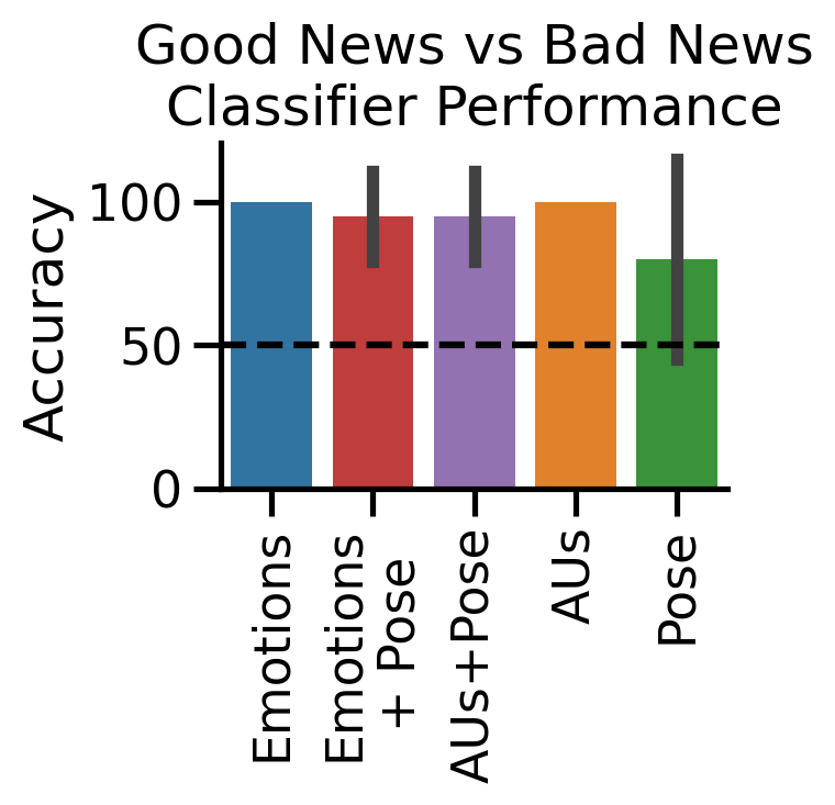
5.5 Decoding condition from facial features

We can easily perform an analysis just like Watson et al, by training a LinearDiscriminantAnalysis (LDA) decoder to classify which condition a video came from based on average AU and headpose detections.

To do this we can use the .predict() which behaves just like .regress() but also requires a sklearn Estimator. We can use keyword arguments to perform 10-fold cross-validation to test the accuracy of each decoder:

from sklearn.discriminant_analysis import LinearDiscriminantAnalysis
from sklearn.preprocessing import (
    StandardScaler,
)  # always a good idea to normalize your features!
from sklearn.pipeline import make_pipeline

# List of different models we'll train
feature_list = ["emotions", "aus", "poses", "emotions,poses", "aus,poses"]
results = []
models = {}

for features in feature_list:

    # .predict is just like .regress, but this time session is our y.
    model, accuracy = by_condition.predict(
        X=features,
        y="sessions",
        model=make_pipeline(StandardScaler(), LinearDiscriminantAnalysis()),
        cv_kwargs={"cv": 10},
    )

    # Save the model
    models[features] = model

    # Save the performance for plotting
    results.append(
        pd.DataFrame(
            {"Accuracy": accuracy * 100, "Features": [features] * len(accuracy)}
        )
    )
    # Print performance
    print(
        f"{features} model accuracy: {accuracy.mean()*100:.3g}% +/- {accuracy.std()*100:.3g}%"
    )

# Concat results into a single dataframe and tweak column names
results = pd.concat(results).assign(
    Features=lambda df: df.Features.map(
        {
            "emotions": "Emotions",
            "poses": "Pose",
            "aus": "AUs",
            "emotions,poses": "Emotions\n+ Pose",
            "aus,poses": "AUs+Pose",
        }
    )
)
# Plot it
# with sns.plotting_context("talk", font_scale=1.8):
f, ax = plt.subplots(1, 1, figsize=(3.75,4));
ax = sns.barplot(
    x="Features",
    y="Accuracy",
    errorbar="sd",
    dodge=False,
    hue="Features",
    data=results,
    ax=ax,
    order=["Emotions", "Emotions\n+ Pose", "AUs+Pose", "AUs", "Pose"],
);
ax.get_legend().remove();
ax.set_title("Good News vs Bad News\nClassifier Performance");
ax.set(ylabel="Accuracy", xlabel="");
sns.despine();
plt.axhline(y=50, ls="--", color="k");
plt.xticks(rotation=90);
plt.tight_layout();

plt.savefig('./fig_maker/decoding_acc.pdf', bbox_inches='tight');

emotions model accuracy: 100% +/- 0%
aus model accuracy: 100% +/- 0%
poses model accuracy: 80% +/- 33.2%
emotions,poses model accuracy: 95% +/- 15%
aus,poses model accuracy: 95% +/- 15%

5.5.1 Visualizing decoder weights

Using what we learned in the previous tutorial, we can visualize the coefficients for any models that used AU features. This allows us to “see” the underlying facial expression that the classifier learned!

from feat.plotting import plot_face

plot_face(
    au=models['aus'][1].coef_.squeeze(), # the LDA coefs from the AUs pipeline model
    feature_range=(0, 1),
    muscles={"all": "heatmap"},
    title="Expression reconstructed from\nAU classifier weights",
    title_kwargs={'wrap':False}
);
sns.despine(left=True,bottom=True);

plt.savefig('./fig_maker/weights.pdf', bbox_inches='tight');

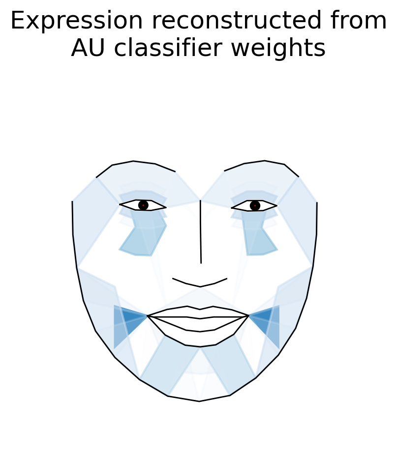
Even cooler we can animate that face expression to emphasize what’s changing. Here we start from a neutral face:

from feat.plotting import animate_face

animation = animate_face(
    end=models['aus'][1].coef_.squeeze(), # same as before
    feature_range=(0, 1),
    muscles={'all': 'heatmap'},
    title="Good vs Bad News Classifier Weights",
    save="weights.gif",
)

5.6 Time-series analysis

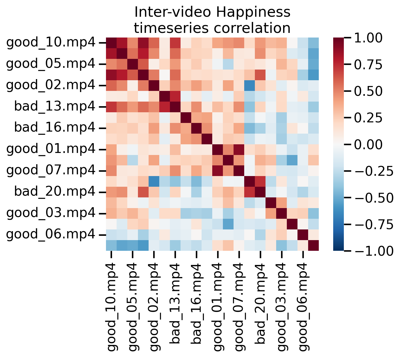
Finally we might be interested in looking the similarity of the detected features over time. We can do that using the .isc() method which takes a column and metric to use. Here we compare detected happiness between all pairs of videos.

We use some helper functions to cluster, sort, and plot the correlation matrix. Warmer colors indicate a pair of videos elicited more similar detected Happiness over time. We see that some videos show high-correlation in-terms of their detected happiness over-time. This is likely why the classifier above was able to decode conditions so well.

# ISC returns a video x video pearson correlation matrix
isc = fex.isc(col = "happiness", method='pearson')

def cluster_corrs(df):
    """Helper to reorder rows and cols of correlation matrix based on clustering"""

    import scipy.cluster.hierarchy as sch

    pairwise_distances = sch.distance.pdist(df)
    linkage = sch.linkage(pairwise_distances, method="complete")
    cluster_distance_threshold = pairwise_distances.max() / 2
    idx_to_cluster_array = sch.fcluster(
        linkage, cluster_distance_threshold, criterion="distance"
    )
    idx = np.argsort(idx_to_cluster_array)
    return df.iloc[idx, :].T.iloc[idx, :]

def add_cond_to_ticks(ax):
    """Helper to add condition info to each tick label"""
    xlabels, ylabels = [], []
    for xlabel, ylabel in zip(ax.get_xticklabels(), ax.get_yticklabels()):
        x_condition = video2condition[xlabel.get_text()]
        y_condition = video2condition[ylabel.get_text()]
        x_new = f"{x_condition[:-4]}_{xlabel.get_text().split('.csv')[0][1:]}"
        y_new = f"{y_condition[:-4]}_{ylabel.get_text().split('.csv')[0][1:]}"
        xlabels.append(x_new)
        ylabels.append(y_new)

    ax.set_xticklabels(xlabels);
    ax.set_yticklabels(ylabels);
    return ax

# Plot it
ax = sns.heatmap(
    cluster_corrs(isc),
    cmap="RdBu_r",
    vmin=-1, vmax=1,
    square=True,
)

ax = add_cond_to_ticks(ax)

ax.set(xlabel="", ylabel="", title="Inter-video Happiness\ntimeseries correlation");
plt.savefig('./fig_maker/isc.pdf', bbox_inches='tight');